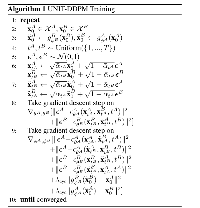
Durham University

所有图片均来源于原论文

Motivation

  • Image to Image任务有时不能保证两个域之间的图片是成对的,比如图像风格转换,一张照片可能找不到与其对应的莫奈风格的画。
  • GAN的方式存在模式崩溃等训练不稳定的情况(已经是老生常谈的话题了🥱)。
  • 因此提出一种类似于CycleGAN的基于扩散模型(DDPM)的方式。

Contribution

  • 基于双域马尔可夫链的生成模型,介绍了一种马尔可夫过程的I2I转换方法,该方法近似源域和目标域的数据分布,使它们相互关联。
  • 不需要对抗训练,模型能根据各种噪声水平的扰动生成捕捉高频变化的真实输出。
  • 马尔科夫链蒙特卡罗采样(Markov Chain Monte Carlo Sampling)的新用途——所提出的采样算法可以根据未配对的源域图像来合成目标域图像。

Methods

  • 原始的DDPM是无监督的,生成条件也只与上一步生成的结果有关,因此核心目标之一就是讲目标域的图像糅合到训练与采样的过程。
  • (需要DDPM相关的理论😁)

Model Structure

  • 模型架构没有什么特别的修改,与基本的DDPM模型一样,都是基于U-net来预测噪声的分布。
image-20230315134020457
  • 归一化改用了Batch_norm,其余的参数设置与DDPM相同。

Training

  • 给定一个源域x0AXA\mathbf{x}_{0}^{A} \in \mathcal{X}^{A}与目标域x0BXB\mathbf{x}_{0}^{B} \in \mathcal{X}^{B},我们需要一个转换模型将其联系起来,即可以做到从A转换到B(反之亦然),原文中使用了DSM模型作为gφ()g_{\varphi^*}^{*}(*),比如x~0B=gϕAA(x0A)\tilde{\mathbf{x}}_{0}^{B}=g_{\phi^{A}}^{A}\left(\mathbf{x}_{0}^{A}\right)以及x~0A=gϕBB(x0B)\tilde{\mathbf{x}}_{0}^{A}=g_{\phi^{B}}^{B}\left(\mathbf{x}_{0}^{B}\right)

  • 反向过程表示为pθAAp_{\theta^{A}}^{A}与$ p_{\theta^{B}}^{B}$,我们要将每一步加入另一个域的图像进行监督,即将反向过程概率表示为:

    pθ(xt1xt,x~t)p_{\theta^{*}}^{*}\left(\mathbf{x}_{t-1}^{*} \mid \mathbf{x}_{t}^{*}, \tilde{\mathbf{x}}_{t}^{*}\right)

    包括pθAA(xt1AxtA,x~tB)p_{\theta^{A}}^{A}\left(\mathbf{x}_{t-1}^{A} \mid \mathbf{x}_{t}^{A}, \tilde{\mathbf{x}}_{t}^{B}\right)pθBB(xt1BxtB,x~tA)p_{\theta^{B}}^{B}\left(\mathbf{x}_{t-1}^{B} \mid \mathbf{x}_{t}^{B}, \tilde{\mathbf{x}}_{t}^{A}\right)

  • 针对于反向过程的损失将变为:

    Lθ(θA,θB)=Et,x0A,ϵ[ϵϵθAA(xt(x0A,ϵ),x~tB,t)2]+Et,x0B,ϵ[ϵϵθBB(xt(x0B,ϵ),x~tA,t)2]\begin{array}{l} \mathcal{L}_{\theta}\left(\theta^{A}, \theta^{B}\right)= \\ \quad \mathbb{E}_{t, \mathbf{x}_{0}^{A}, \boldsymbol{\epsilon}}\left[\left\|\boldsymbol{\epsilon}-\epsilon_{\theta^{A}}^{A}\left(\mathbf{x}_{t}\left(\mathbf{x}_{0}^{A}, \boldsymbol{\epsilon}\right), \tilde{\mathbf{x}}_{t}^{B}, t\right)\right\|^{2}\right] \\ \quad+\mathbb{E}_{t, \mathbf{x}_{0}^{B}, \boldsymbol{\epsilon}}\left[\left\|\boldsymbol{\epsilon}-\epsilon_{\theta^{B}}^{B}\left(\mathbf{x}_{t}\left(\mathbf{x}_{0}^{B}, \boldsymbol{\epsilon}\right), \tilde{\mathbf{x}}_{t}^{A}, t\right)\right\|^{2}\right] \end{array}

  • 而对于DSM的参数ϕA\phi^{A}ϕB\phi^{B},固定反向过程中的参数θ\theta^*,最小化损失为:

    Lϵϕ(ϕA,ϕB)=Et,x0B,ϵ[ϵϵθAA(xt(gϕBB(x0B),ϵ),xt(x0B,ϵ),t)2+ϵϵθBB(xt(x0B,ϵ),gϕBB(xt(x0B),ϵ),t)2]+Et,x0A,ϵ[ϵϵθBB(xt(gϕAA(x0A),ϵ),xt(x0A,ϵ),t)2+ϵϵθAA(xt(x0A,ϵ),gϕAA(xt(x0A),ϵ),t)2]\begin{array}{l} \mathcal{L}_{\epsilon^{\phi}}\left(\phi^{A}, \phi^{B}\right)= \\ \mathbb{E}_{t, \mathbf{x}_{0}^{B}, \boldsymbol{\epsilon}}\left[\left\|\boldsymbol{\epsilon}-\epsilon_{\theta^{A}}^{A}\left(\mathbf{x}_{t}\left(g_{\phi^{B}}^{B}\left(\mathbf{x}_{0}^{B}\right), \boldsymbol{\epsilon}\right), \mathbf{x}_{t}\left(\mathbf{x}_{0}^{B}, \boldsymbol{\epsilon}\right), t\right)\right\|^{2}\right. \\ \left.\quad+\left\|\boldsymbol{\epsilon}-\epsilon_{\theta^{B}}^{B}\left(\mathbf{x}_{t}\left(\mathbf{x}_{0}^{B}, \boldsymbol{\epsilon}\right), g_{\phi^{B}}^{B}\left(\mathbf{x}_{t}\left(\mathbf{x}_{0}^{B}\right), \boldsymbol{\epsilon}\right), t\right)\right\|^{2}\right] \\ +\mathbb{E}_{t, \mathbf{x}_{0}^{A}, \boldsymbol{\epsilon}}\left[\left\|\boldsymbol{\epsilon}-\epsilon_{\theta^{B}}^{B}\left(\mathbf{x}_{t}\left(g_{\phi^{A}}^{A}\left(\mathbf{x}_{0}^{A}\right), \boldsymbol{\epsilon}\right), \mathbf{x}_{t}\left(\mathbf{x}_{0}^{A}, \boldsymbol{\epsilon}\right), t\right)\right\|^{2}\right. \\ \left.\quad+\left\|\boldsymbol{\epsilon}-\epsilon_{\theta^{A}}^{A}\left(\mathbf{x}_{t}\left(\mathbf{x}_{0}^{A}, \boldsymbol{\epsilon}\right), g_{\phi^{A}}^{A}\left(\mathbf{x}_{t}\left(\mathbf{x}_{0}^{A}\right), \boldsymbol{\epsilon}\right), t\right)\right\|^{2}\right] \end{array}

    对于这个损失函数,还需要引进规范化,称为Cycle-consistency Loss,被定义为:

    Lcycϕ(ϕA,ϕB)=Ex0B[gϕAA(gϕBB(x0B))x0B1]+Ex0A[gϕBB(gϕAA(x0A))x0A1]\mathcal{L}_{\mathrm{cyc}^\phi}(\phi^A,\phi^B)= \mathbb{E}_{\mathbf{x}_0^B}[\|g_{\phi^A}^A(g_{\phi^B}^B(\mathbf{x}_{0}^B))-\mathbf{x}^B_0\|_1] \\ +\mathbb{E}_{\mathbf{x}_0^A}[\|g_{\phi^B}^B(g_{\phi^A}^A(\mathbf{x}_{0}^A))-\mathbf{x}^A_0\|_1]

    最后,针对于DSM的参数的损失:

    Lϕ(ϕA,ϕB)=Lϵϕ(ϕA,ϕB)+λcycLcycϕ(ϕA,ϕB)\mathcal L_\phi(\phi^A,\phi^B)=\mathcal L_{\epsilon^\phi}(\phi^A,\phi^{B})+\lambda_{\mathrm{cyc}}\mathcal L_{\mathrm{cyc}^\phi}(\phi^{A},\phi^{B})

    其中,λcyc\lambda_{\mathrm{cyc}}是权重。

  • 其余的训练过程与DDPM相同,整体的训练流程:

    image-20230315122805925
  • 算法过程:

    image-20230315150135482

Sampling

  • 采样的过程不再需要DSM进行转换,因此后向过程中只有参数θ\theta^{*}起作用。

  • 假设我们要做A➡️B的转换,那么我们的从一幅纯高斯噪声图带噪声的A域的图像开始。

  • 生成的过程以带噪声的A域图像(从T到任意时刻tr[1,T]t_r \in[1,T]的正向加噪生成)为条件,然后从此时刻trt_r开始反向过程,重新生成图片,将trt_r称为Release time(释放时间🤔)。

  • 从域A转移到域B的过程表述为:

    x^t1B=μθB(x^tB,x^tA,t)+ΣθB(xt,t)ϵB\hat{\mathbf{x}}_{t-1}^B=\mu_{\theta^B}(\hat{\mathbf{x}}_t^B,\hat{\mathbf{x}}_t^A,t)+\Sigma_{\theta^B}(\mathbf{x}_t,t)\epsilon^B

    x^t1A={α^tAx0A+1αˉtAϵA(t>tr)μθA(x^tA,x^tB,t)+ΣθA(xtA,t)ϵB(ttr)\hat{\mathbf{x}}^A_{t-1}=\left\{ \begin{array}{ll} \sqrt{\hat{\alpha}_tA}\mathbf{x}^A_0+\sqrt{1\bar{\alpha}_tA}\boldsymbol{\epsilon}^A&(t>t_r)\\ \mu_{\theta^A}(\hat{\mathbf{x}}_t^A,\hat{\mathbf{x}}_t^B,t)+\Sigma_{\theta^A}(\mathbf{x}_t^A,t)\epsilon^B & (t \le t_r) \end{array}\right.

    其中,x^TB,ϵA,ϵBN(0,I)\hat{\mathbf{x}}^B_T,\epsilon^A,\epsilon^B\sim\mathcal{N}(0,\mathbf{I})

  • 整体过程:

    image-20230315140734418
  • 算法流程:

    image-20230315152955317

Ablation Study

  • 文章中的消融实验主要针对了采样过程中的Release time。FID分数的变化依赖于数据集,一些数据集上受Release time影响小,可能归因于发布时间变化的微小差异。

  • 这一结果表明,Release time超参数的调整依赖于数据集。

    image-20230315140801737

Results

  • 得到结果是很好的:

    image-20230315133928794

  • 但是代码没开源😶‍🌫️

  • 而且目前只能在很小分辨率的图像上有很好的效果。